Dynamic range, often abbreviated simply as DR, is a very important parameter in analog signals and circuits, as well as digital systems and associated data. In simplest terms, it is the ratio between the largest valid analog signal (or digital number) in a system and the smallest viable one, Figure 1. If a design's dynamic range is less than the anticipated DR of the analog system or digitized data that it is supposed to handle, the result will be severe shortcomings in performance (analog circuits) or numerical errors (digital processing) due to overrange (signal/number too big) or underrange (signal/number too small). Conversely, if the system can handle a much wider DN than the signals require, much of the system resolution will be wasted and the signal/data will not be seen in sufficient detail.
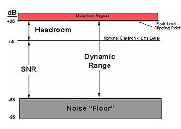 Dynamic range is the ratio between the largest and smallest signal the system can handle, and is often expressed in dB; the smallest is often determined by the system's inherent noise. All captions need to include a source credit. Image source: Analog Devices, Inc.
There are three common ways to quantify and express DR: as a simple numeric ratio, in decibels (dB), or as a binary value; the application will determine which is used. In the real world of sensors or wireless signals, the front-end analog circuitry must handle signals which can span a wide dynamic range of 100 dB or more (that's a span of 100,000:1 or 105:1 for voltage, and 1010:1 for power). Even financial systems must worry about DR, as an accounting system which handles tens of billions of dollars ($10,000,000,000+) may also need to express the amount down to the penny ($0.01) or perhaps fractions of a penny. Due to the wide ratio needed, most circuit designs discuss DR in decibels (dB), using a base 10 logarithmic scale:
dB (power) = 10 × log10(P1 / P0)
dB (volts) = 20 × log10(V1 / V0)
where P1 / P0 (and V1 / V0) are ratios between the largest and smallest power (and voltage) values, respectively. For example, 100 dB represents a factor of 100,000 in amplitude (usually volts) and a factor 10,000,000,000 in power.
For digital systems, or analog systems with a digital aspect, the scale of bits is often used, with every additional bit in the binary representation doubling the DR and increasing DR by 6 dB (voltage). For example, a four-bit binary number represents the 16 distinct values 0000 through 1111, while the five-place binary number represents the 32 values 00000 though 11111.
DR and system resolution
How much DR do you need? The answer, of course, "it depends." The factors on which it depends include the application, the signal source, and the intended signal processing effort in the analog and digital domains. A DR of 60 dB is a fairly low value; many systems are in the 80-100 dB range, and a large number of designs, especially in the wireless/optical area where the signal channel is largely beyond control of the receiver, can reach 120 and even higher dB values. Some typical DR ranges include:
- Weight scale: 0.1 pound to 500 pounds = 5000:1 = 74 dB = 12.3 bits
- Human ear: minimum audible level is 2 ×10⁻⁵ Pa defined as 0 dB; pain level is around 110 dB or 106:1 = 23.3 bits
- Power/energy meter (current): 0.05 to 200 A = 4000:1 = 72 dB = 12 bits
- Temperature: 0.1⁰ from 0⁰ to 100⁰ = 1000:1 = 60 dB = 10 bits
- Received Optical or RF signal amplitude (voltage): 1 μV to 100 mV = 100,000:1 = 100 dB = 16.6 dB
The challenge for design engineers is that getting sufficient DR is difficult in many cases, requiring high-performance components, understanding noise and circuit perturbations, attention to power-supply rail issues, and even costlier components. However, it many cases, what is needed is not so much wide DR as much as high resolution in some areas of the overall signal range.
Consider a weigh scale which must resolve to 0.1 pound over a 500-pound range, which is a 5000:1 ratio, equivalent to 74 dB or 12 bits. This is actually a fairly modest requirement with today's systems and may be sufficient is all that you are doing is weighing packages.
Controlling gain can reduce pain
If what you really want to see are slight changes around a measured nominal point in the range, you may instead be looking for changes of 1/100 pound (0.01 pound) across the 500-pound range, which is a 50,000:1 DR, or 94 dB/15.6 bits. While this is achievable, it is much more challenging than the original 74-dB requirement. Not only are higher-resolution converters more costly, they are harder to actually implement in a design where they can achieve their full potential.
 By continually adjusting the gain so the signal stays within a defined range, the system can handle signals with much-wider dynamic range than the basic circuitry can tolerate, making much better use of the available dynamic range. All captions need to include a source credit. Image source: Researchgate.net.Therefore, instead of looking for higher resolution across the entire range, the solution which many engineers prefer is to use valuable gain amplifier (VGA) along with gain ranging and scaling, Figure 2. This technique is especially effective for signals at the low end of the range, where internal system noise can swamp the desired signal and negate actual resolution. Looking for ±0.01 pound changes around a 0.1-pound nominal signal is much more difficult than seeing those same for ±0.01 pound variations around a nominal nine-pound signal.
For convenience, assume 0 V equals 0 pounds and 10 V equals 500 pounds; thus a 0.01 pound change is ±0.0002 V. In gain ranging, when the nominal signal falls below some predefined threshold, such as 0.5-V (25 pounds), the VGA is instructed b the system microcontroller to increase its gain to ×10 (for example), so the signal of interest is ten times larger, and so are the changes for which you are looking (now ±0.002 V). This larger change is far easier to "see" accurately and makes better use of the converter's maximum resolution. Then between 1- and 2-V nominal voltage, the gain is decreased to x5, which still increase the changes to 0.001 V.
Gain-ranging and scaling is not just a viable technique for relatively slow, static signals such as weight scales. Even fast-changing RF signals with DRs of 100 dB and more often use a VGA to dynamically adjust front-end gain and so reduce the DR demands and the associated component cost and circuit complexity, while maintaining performance at the low-amplitude end where internal noise will be an issue.
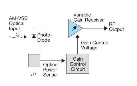 Automatic gain control uses a closed loop to adjust gain depending on signal strength; here shown for an optical-to-electronic signal converter. All captions need to include a source credit. Image source: Lightwave.
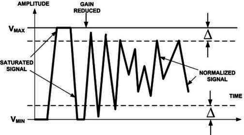
 As the AGC control voltage "kicks in" and the gain is adjusted, the signal goes from extreme to a more bounded value. Image source: Analog Devices, Inc.
However, unlike the weigh scale where the gain is adjusted by a microcontroller after it makes an approximate measurement, the RF signal channel does it using a closed loop of analog circuitry in most cases. This automatic gain control (AGC) circuit senses the received front-end power level and develops a control signal which increases gain when the received signal strength (RSS) is low, and decreases gain when the RSS is higher, Figure 3 and Figure 4. In this way, the usefulness and credibility of the actual available DR is put to best use, especially when the signal's DR is greater than that of the circuitry and its internal noise.
Going log, beyond linear
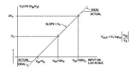
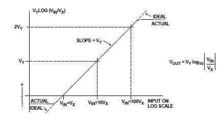 In a log amplifier, the output is linearly proportional to the logarithm (base 10) of the input; as a result, a very wide dynamic range of inputs can be handled with a modest output-voltage span. Image source: Analog Devices, Inc.To manage wide DR and gain-setting even more effectively, a logarithmic amplifier is often used. These "log amps" produce an output that is proportional to the common (base 10) logarithm of the input signal amplitude; this response is described as being linear-in-dB, Figure 5. Some log amps can handle dynamic ranges of 140 and dB and beyond, and work well with converters of modest resolution such as 16-bit, high-speed devices.
A prime reason to use variable gain and ranging rather than just go to a higher-resolution A/D or D/A converter to achieve the DR you need is the reality of system and converter noise floor. Although the converter design may legitimately be rated at some number of bits of resolution (and thus DR), the effective number of bits (ENOB) is lower to due noise and imperfections. The basic formula is ENOB = (SNR – 1.76)/6.02 dB (Reference 1 explains the source of this formula). Therefore, a 12-bit A/D converter with modest imperfections may have an SNR of 65 dB, resulting in an ENOB of 10.5 bits, which is less than the original 12-bit rating, at 10.5 bits × 6 dB/bit= 63 dB rather than 12 bits × 6 dB/bit= 73 dB.
When doing any design, it is important to keep the DR objectives and system realities in mind, and compare the two. If they do not match, either the DR requirement will have to be relaxed, or techniques will needed to maximum the achievable DR from available components, Fortunately, this is such a common situation that there are many standard, tested, and vetted techniques for maximizing DR and associated resolution, range, and ENOB while managing cost, power consumption, and layout risk.
References